Section 11.4 Plotting Surfaces
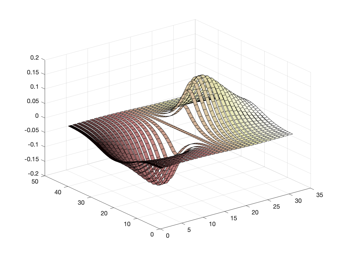
So far we have focused on graphing curves in space. We’ll now turn to surfaces and MATLAB’s capabilities to visualize them. Many surfaces in three-dimensional space can be described as functions of two variables. Here is an example of a surface:
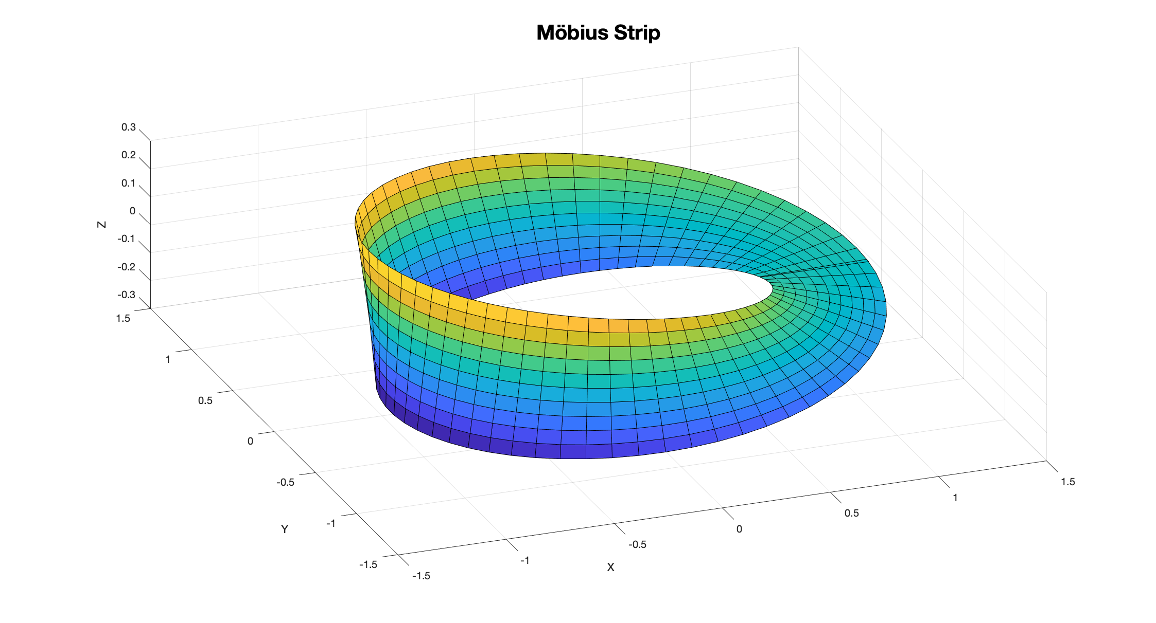
MATLAB has several built-in functions to plot surfaces. A surface is specified by its z-values on a grid of \(x,y\) values. Here is what such a grid might look like:
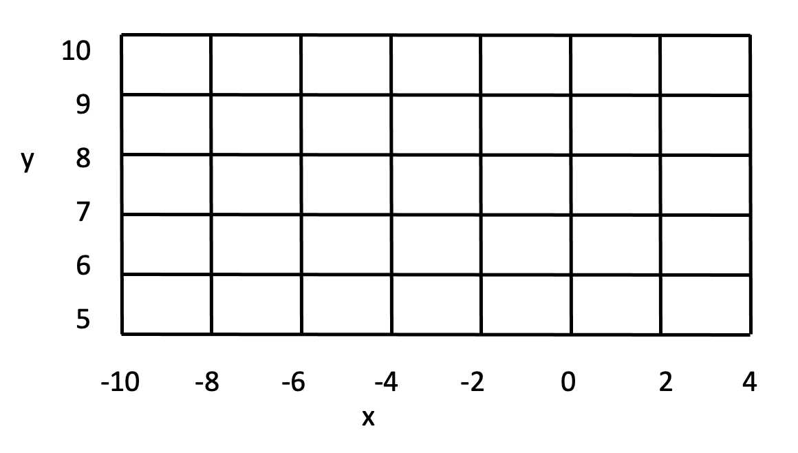
We’ll shortly learn how to easily create such a grid in MATLAB. Once this grid is created, here are the steps to display your surface. MATLAB offers several options to help the viewer visualize the 3-dimensional nature of the plot. Two of these options are mesh and surface plots. These 3D plots can be used to graph surfaces that are given in the following form:
\begin{equation*}
z = f(x,y)
\end{equation*}
where
-
\(x\) and \(y\) are the independent variables
-
z is the dependent variable
Within a given domain the value of \(z\) can be calculated for any combination of \(x\) and \(y\text{.}\)
Mesh and surface plots are created in 3 steps:
-
create a grid in the x-y plane that covers the whole domain
-
calculate the value of z at each point of the grid
-
create a plot
Here are the details for these three steps:
Subsection 11.4.1 Step 1
Create a grid in the x-y plane that covers the whole domain
The desired grid is a set of points in the x-y plane in the domain of the function. Each point on the grid has an x-coordinate and a y-coordinate:
\begin{equation*}
(X,Y) = \begin{bmatrix}(-10,10) & (-8,10) & (-6,10) & \cdots & (2,10) & (4,10) \\
(-10, 9) & (-8, 9) & (-6, 9) & \cdots & (2, 9) & (4, 9) \\
(-10, 8) & (-8, 8) & (-6, 8) & \cdots & (2, 8) & (4, 8) \\
\vdots & \vdots & \vdots & \ddots & \vdots & \vdots \\
(-10, 5) & (-8, 5) & (-6, 5) & \cdots & (2, 5) & (4, 5)
\end{bmatrix}
\end{equation*}
We’ll therefore need to create two matrices of the same size: one matrix that contains all of the x-coordinates of all points, and one matrix that contains all of the y-coordinates.
\begin{equation*}
X = \begin{bmatrix}-10 & -8 & -6 & \cdots & 2 & 4 \\
-10 & -8 & -6 & \cdots & 2 & 4 \\
-10 & -8 & -6 & \cdots & 2 & 4 \\
\vdots & \vdots & \vdots & \ddots & \vdots & \vdots \\
-10 & -8 & -6 & \cdots & 2 & 4
\end{bmatrix}, \text{ and }
Y = \begin{bmatrix}10 & 10 & 10 & \cdots & 10 & 10 \\
9 & 9 & 9 & \cdots & 9 & 9 \\
8 & 8 & 8 & \cdots & 8 & 8 \\
\vdots & \vdots & \vdots & \ddots & \vdots & \vdots \\
5 & 5 & 5 & \cdots & 5 & 5
\end{bmatrix}
\end{equation*}
The density of the grid (number of points at which we’ll compute the z-values) is user-defined.
Observe the following properties of the matrices X and Y:
-
Matrix X, which contains the x-coordinates of all the points, has identical rows.
-
Matrix Y, which contains the y-coordinates of all the points, has identical columns.
MATLAB offers the meshgrid command to help you create these matrices. All you need is a vector of the desired x-values in the grid and another vector of the desired y-values. The
meshgrid function then creates the two matrices:
x = -10:2:4;
y = 5:10;
[X,Y] = meshgrid(x,y);
Subsection 11.4.2 Step 2
Calculate the value of z at each point of the grid
Once you have created the matrices X and Y you can do element-by-element calculations with these matrices in order to compute, for each pair of (x,y) values, the corresponding z-coordinate.
Here is an example:
Z = 2.^(-1.5*sqrt(X.^2 + Y.^2)).*cos(0.5*Y).*sin(0.5*X);
The calculated dependent variable z is a also a matrix of the same size as both X and Y.
Subsection 11.4.3 Step 3
Create a plot!
We’ll now take a look at a number of ways to plot your surface.
mesh(X,Y,Z);
% 3D surface, open mesh, color indicates height.
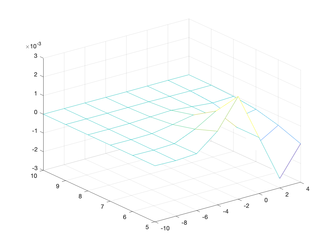
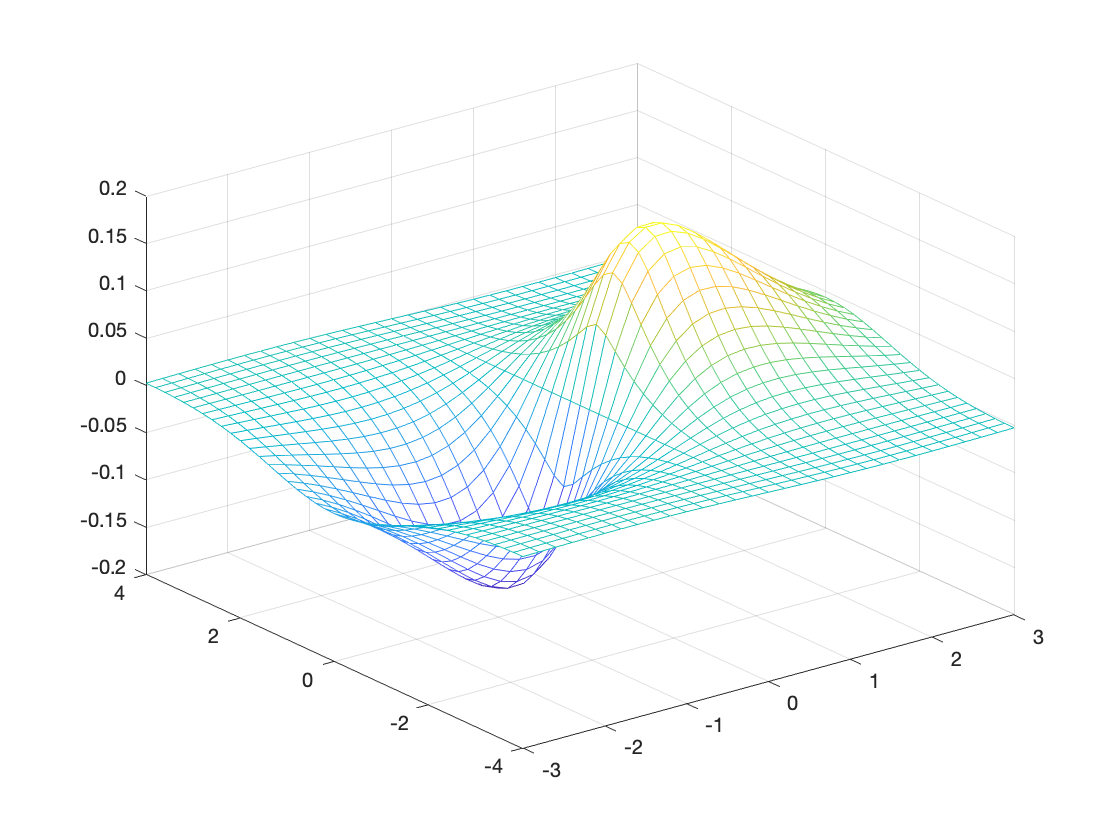
This clearly looks terrible! The mesh is not dense enough and the range of values too large. Here is a better version:
x = -3:.2:3;
y = -4:.2:4;
[X,Y] = meshgrid(x,y);
Z = 2.^(-1.5*sqrt(X.^2 + Y.^2)).*cos(0.5*Y).*sin(0.5*X);
mesh(X,Y,Z);
% 3D surface, open mesh, color indicates height.
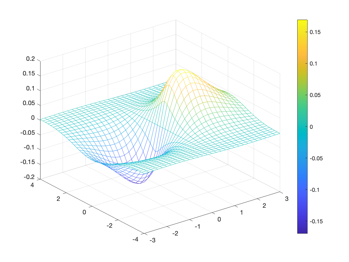
You can display a legend of colors, if you wish, using the built-in function colorbar:
colorbar
% Turns on the colorbar
Below are a number of other options to display your surface:
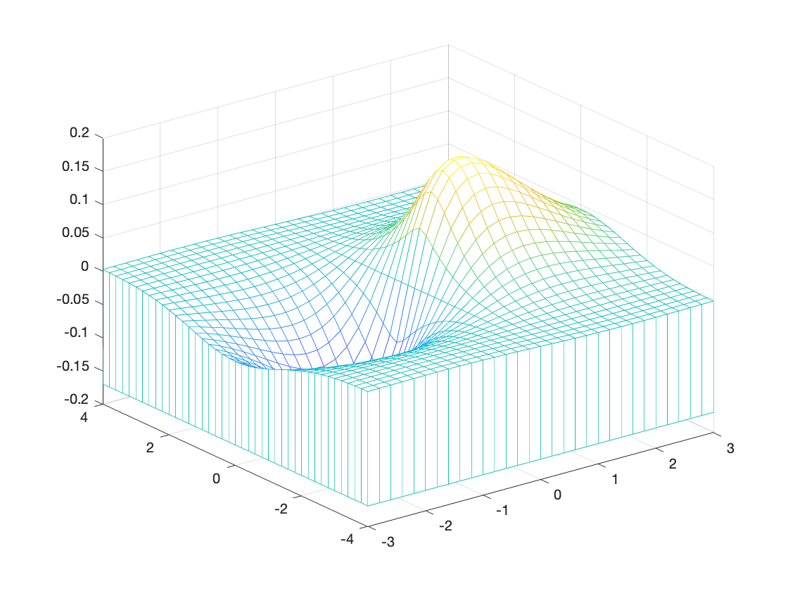
meshz(X,Y,Z);
% 3D surface, open mesh with curtain, color indicates height.
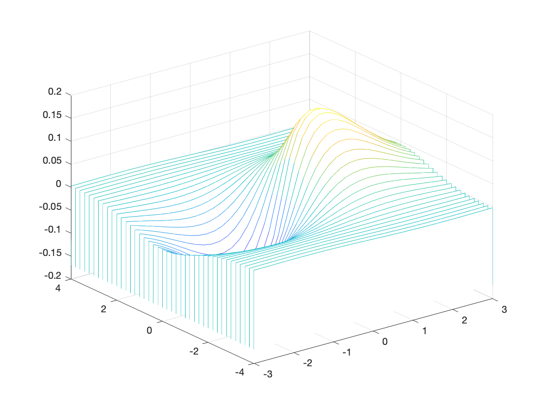
waterfall(X,Y,Z);
% 3D surface, waterfall (lines of constant y).
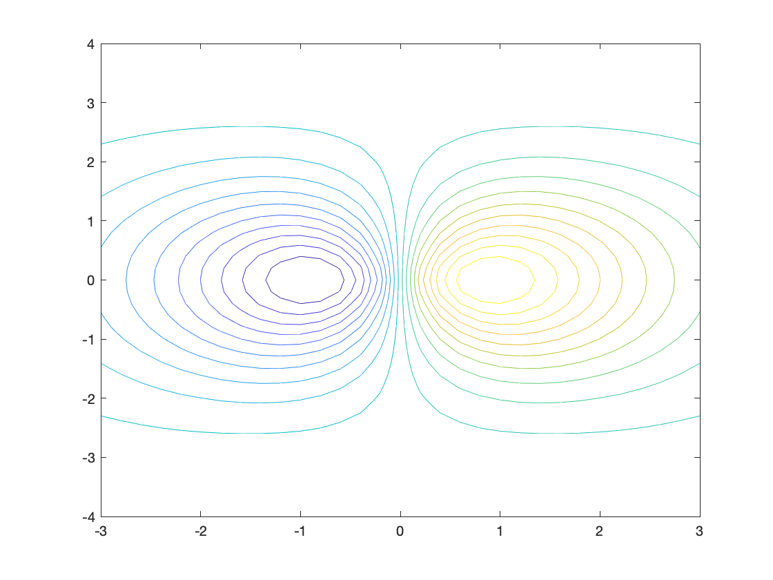
contour(X,Y,Z,n);
% n curves of constant Z value (replace n with a number  of your choice).
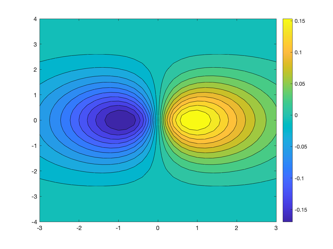
contourf(X,Y,Z,n);
colorbar;
% 2D filled curves of constant Z value.
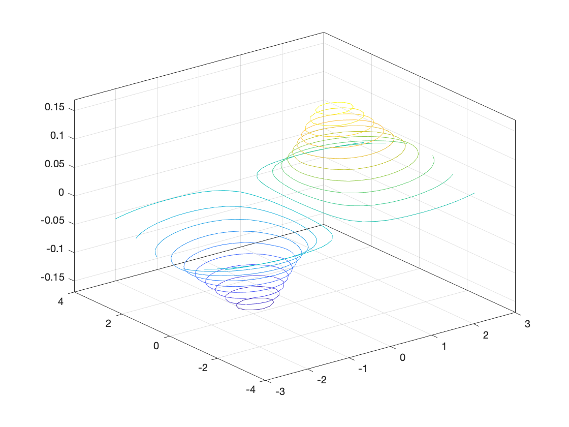
contour3(X,Y,Z,n);
% 3D curves of constant Z value.
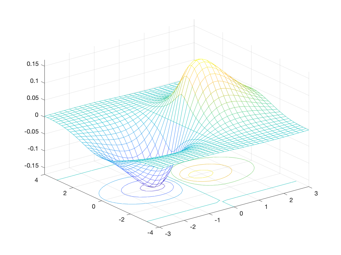
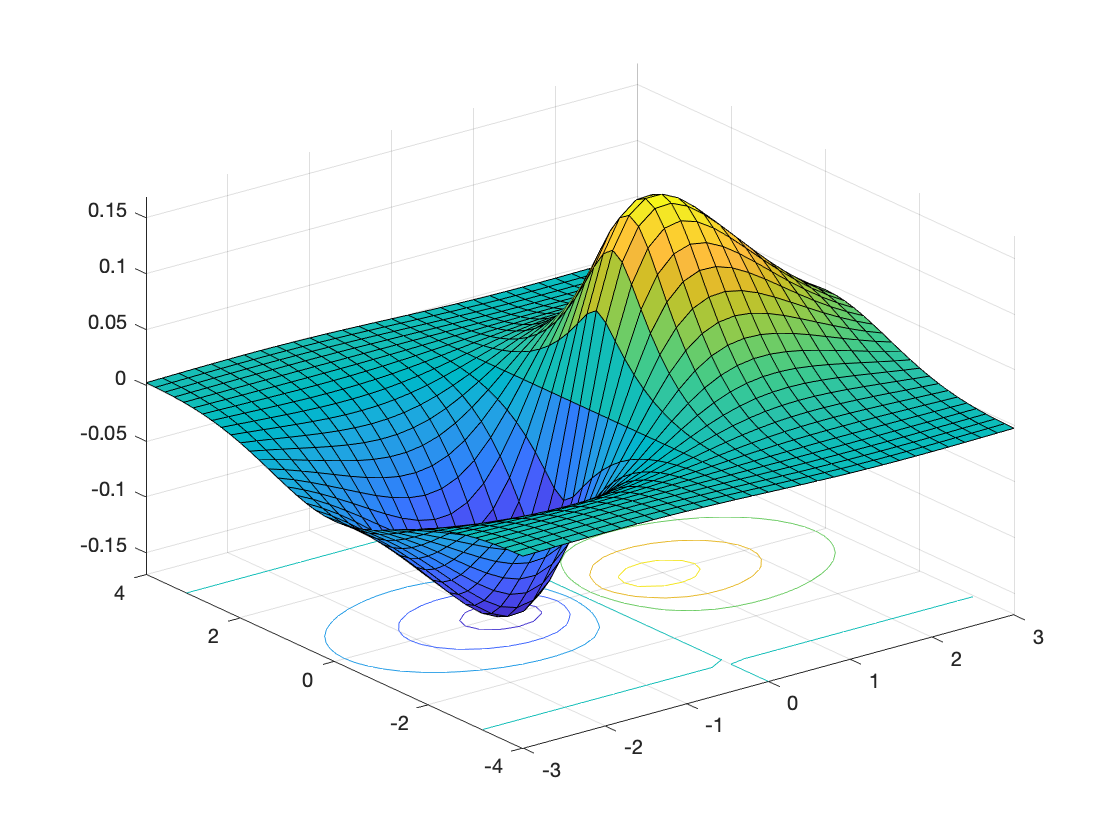
meshc(X,Y,Z);
% Combined mesh and 2D contour.
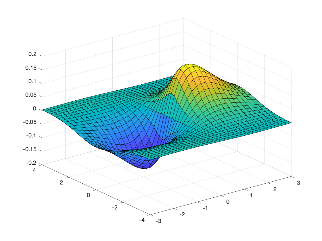
surf(X,Y,Z);
% 3D surface, filled mesh, color indicates height.
surfc(X,Y,Z);
% Combined surface and 2D contour.
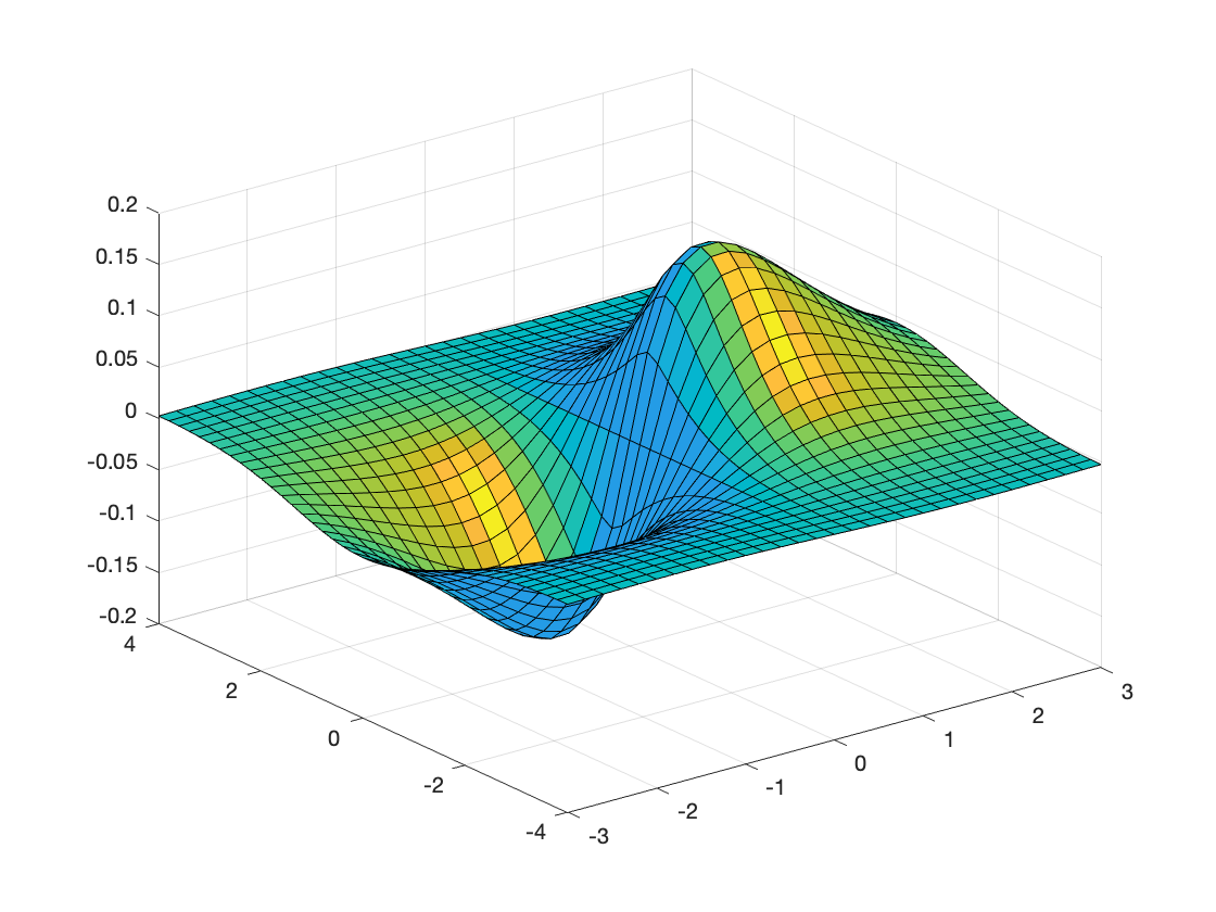
surfl(X,Y,Z);
% Surface with lighting: color indicates intensity.
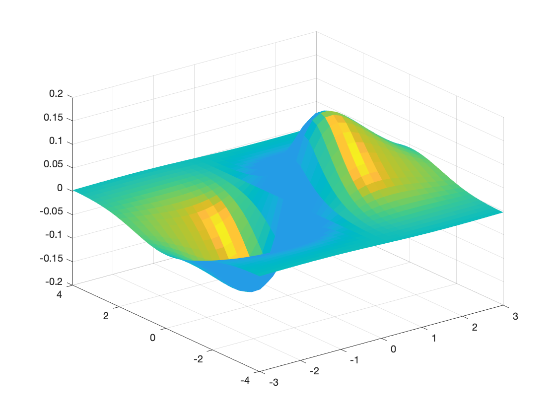
surfl(X,Y,Z);    % Surface with lighting.
shading flat;    % Flat shading removes grid lines.
surfl(X,Y,Z);       % Surface with lighting.
shading interp;     % Interpolated shading looks smoother.
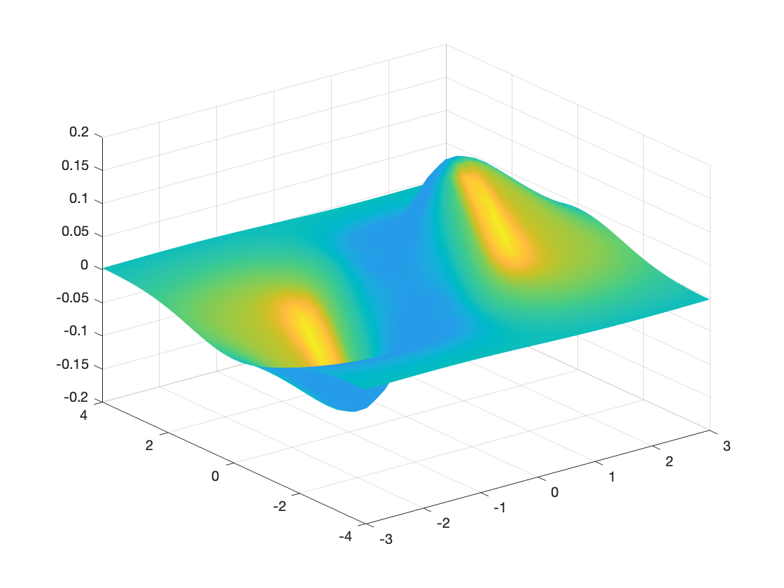
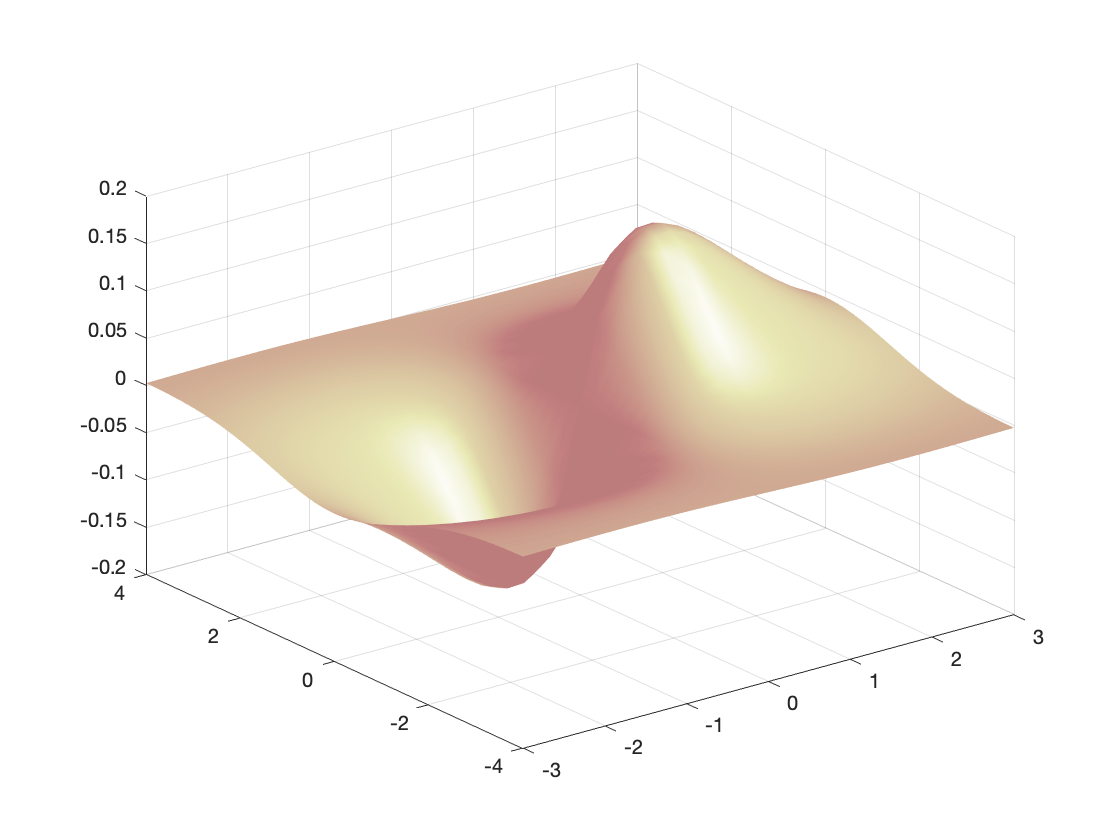
surfl(X,Y,Z);       % Surface with lighting.
shading interp;     % Interpolated shading looks smoother.
colormap pink;
ribbon(Z);
% Surface strips: color indicates strip.
