Section 6.5 Plotting Functions
Plotting a function requires that an array of abscissa values are created first. Next, you evaluate the function at all of these values to give you pairs of (x,y) coordinates to be plotted.
\begin{equation*}
y = 3.5^{-x/2}\,cos(6x)
\end{equation*}
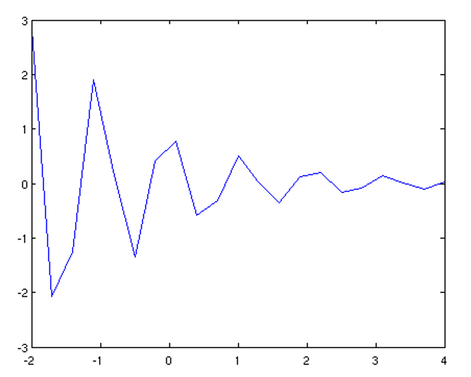
>> x = -2:0.3:4;
>> y = 3.5.^(-0.5*x).*cos(6*x);
>> plot(x,y)

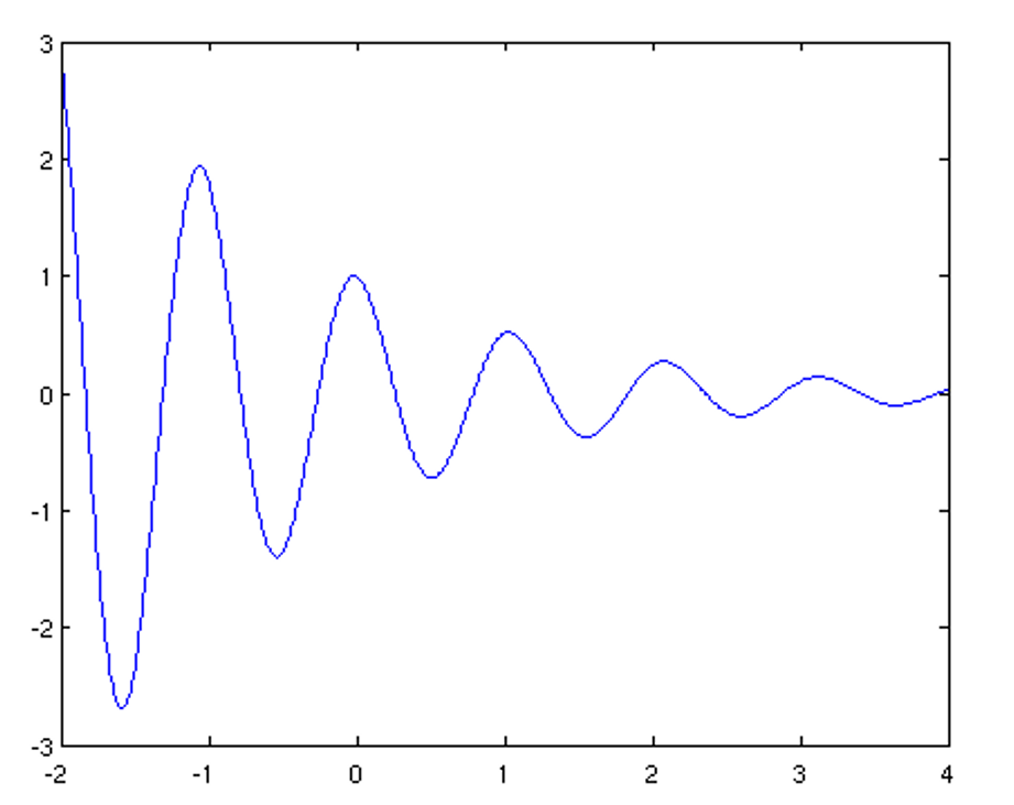
The above plot looks rather edgy but should be looking smooth. What is the problem? MATLAB automatically connects subsequent points of the plot with lines. So if the points are too far apart from each other, the graph will look edgy. It is thus important for plotting a function to choose an array of appropriately spaced abscissa values. Below is a better choice for our example:
\begin{equation*}
y = 3.5^{-x/2}\,cos(6x)
\end{equation*}
>> x = -2:0.01:4;
>> y = 3.5.^(-0.5*x).*cos(6*x);
>> plot(x,y)

Subsection 6.5.1 Using fplot()
Plotting a function of a single variable can be done using the
fplot command:
>> fplot(function, limits, 'line specifiers')
function used to accept a string in which the function to be plotted was specified and so you may still encounter such code. Future releases of MATLAB will no longer accept such input.
We will learn more about functions in the chapter on functions, but for now you can simply accept the following syntax:
@(argument) function
For example,
@(x) x.^2
defines the function \(y = x^2\text{.}\)
limits is either a two element vector specifying the domain of the argument \(\begin{bmatrix}
X_{min}, & X_{max}
\end{bmatrix}\) or a four element vector specifying the domain of x and the limits of y \(\begin{bmatrix}
X_{min}, & X_{max}, & Y_{min}, & Y_{max}
\end{bmatrix}\text{.}\)
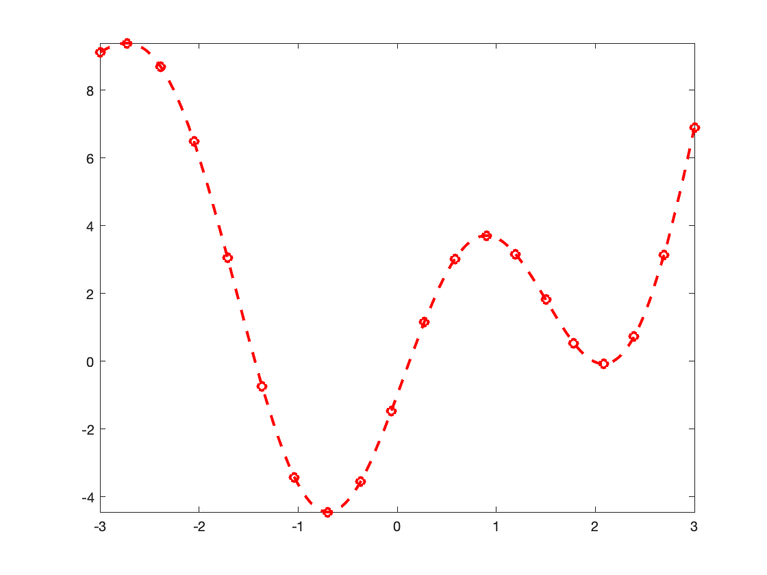
>> fplot(@(x) x.^2+4.*sin(2.*x)-1, [-3,3], '--or', 'linewidth', 2)


