Section 11.2 Simple Line Plots
Rather than being 2-dimensional, a curve can also be situated in space. Once way to describe such a curve is to specify a sequence of \((x,y,z)\) coordinates along that curve and plot all of those points. To do so we use the MATLAB
plot3 command which works exactly like the plot command except for accounting for an extra z-coordinate.
plot3(x,y,z, 'line specifiers', 'PropertyName', ...property value)
\(x, y, z\) must all be vectors of the same size.
Line specifiers and PropertyName/property value pairs are optional and work just like in 2D plotting, see Section 6.3.
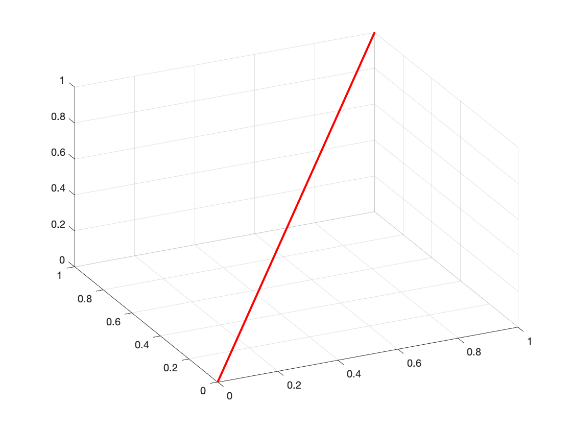
Here is a very simple example: To plot a line in space from the origin \((0,0,0)\) to the point \((1,1,1)\) you could use the following code:
x = 0:.1:1;
y = x;
z = x;
plot3(x,y,z,'linewidth', '2', 'color', 'r')
grid on
The grid command is helpful to the viewer in emphasizing the three-dimensional nature of the plot.

Most 3-dimensional curves are actually given in parametric form: x, y and z are functions of a parameter, t. Here is an example:
t = 0:0.1:6*pi;
x = sqrt(t).*sin(2*t);
y = sqrt(t).*cos(2*t);
z = t;
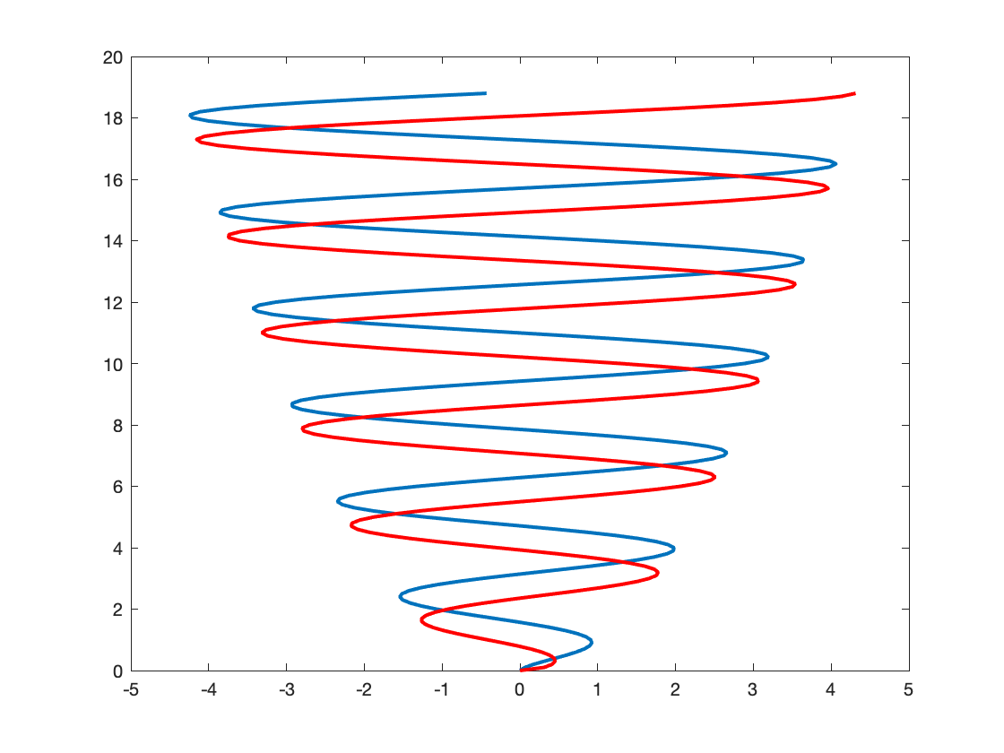
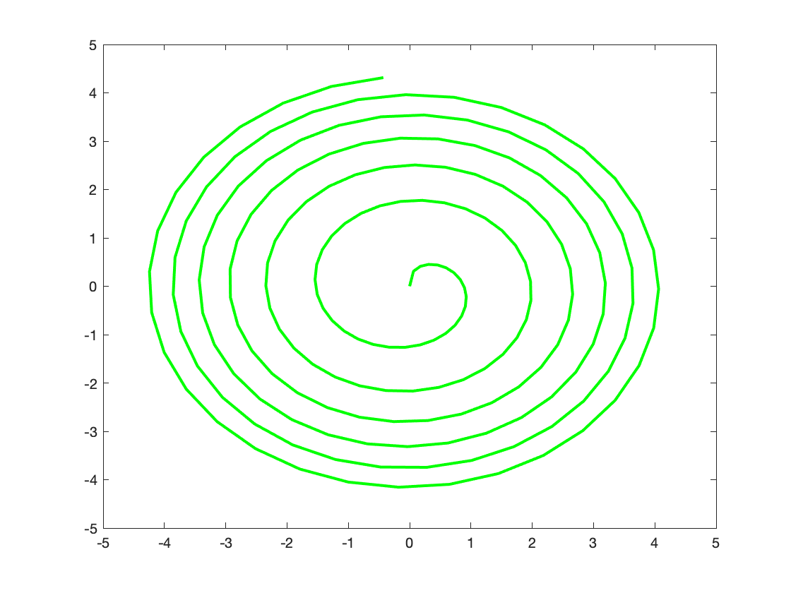
Here, \(x(t), y(t), z(t)\) form a parametric curve. What does it look like? We’ll use the plot3 command below to find out. But you can also think about this on your own first by only looking at the 2-dimensional curves x-versus-t, y-versus-t and x-versus y:
plot(x,t, y,t, 'r', 'linewidth',2);
figure;
plot(x,y,'g', 'linewidth', 2);


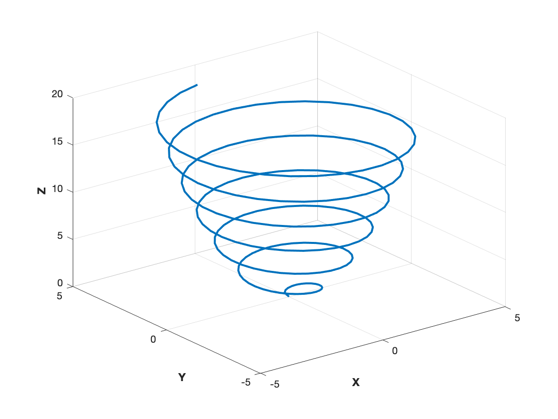
Having seen and thought about these curves will help you predict what the three-dimensional curve looks like. Of course, MATLAB can also do so:
t = 0:0.1:6*pi;
x = sqrt(t).*sin(2*t);
y = sqrt(t).*cos(2*t);
z = t;
plot3(x,y,z, 'linewidth', 2);
xlabel('{\bf X}');
ylabel('{\bf Y}');
zlabel('{\bf Z}');
grid on;


