So far we’ve mostly focused on whether our code and algorithms are correct. But when working with large datasets, it also matters how much work an algorithm has to do. Runtime analysis is our way of estimating how the amount of work (time, memory, …) grows as the input size \(n\) becomes large.
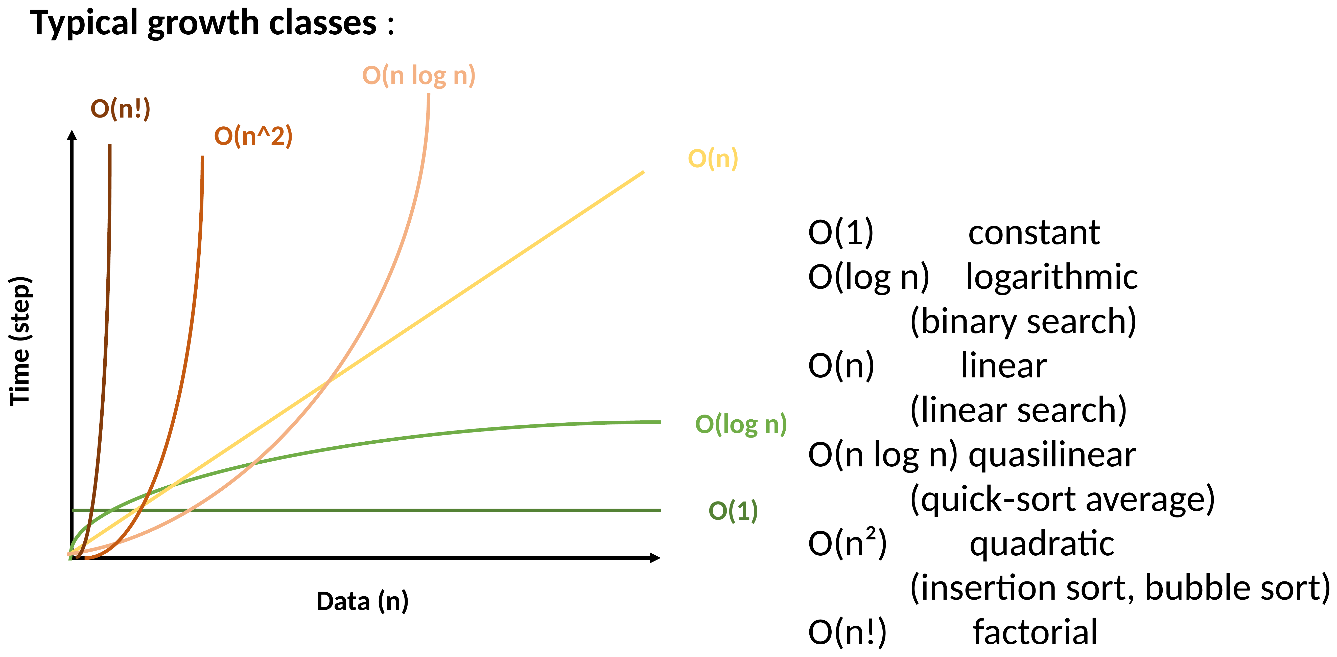
Rather than counting the exact number of operations (which would depend on the specific computer, compiler, and even the specific input), we focus on the dominant term and ignore constant factors and lower-order terms. This is captured by Big-O notation: we say an algorithm runs in \(O(f(n))\) time if, for sufficiently large \(n\text{,}\) the runtime never exceeds \(c \cdot f(n)\) for some constant \(c\text{.}\)
#include <stdio.h>
int main(void) {
    int list[] = {6, -2, 5, 12, 7, 3, 8, 15, -10, 1};
    int n = 10;
    int item, i, found;
    printf("What number are you interested in?");
    scanf("%d", &item);
    i = 0;
    found = 0;
    while(!found && i<n){
        if(list[i] == item){
            found = 1;
        }
        else{
            i++;
        }
    }
    return (0);
}
In the worst case (the item is last, or not present at all) the while loop runs \(n\) times, so linear search is \(O(n)\)— linear time.
#include<stdio.h>
int main(void) {
    int n = 10;
    int i, j, swap;
    int list[] = {759, 14, 2, 900, 106, 77, -10, 8, -3, 5};

    for(j=0; j<n-1; j++){
        for(i=0; i<n-1; i++){
            if(list[i] > list[i+1]){
                swap = list[i];
                list[i] = list[i+1];
                list[i+1] = swap;
            }
        }
    }
    return (0);
}
Here we have two nested loops, each running roughly \(n\) times, so the inner comparison happens roughly \(n^2\) times: bubble sort is \(O(n^2)\)— quadratic time.
Where does QuickSort fit in? On average, each partitioning step is \(O(n)\text{,}\) and the list roughly halves in size each time, giving \(O(n \log n)\) overall— much better than bubble sort’s \(O(n^2)\text{!}\) But in the worst case (for example, an already-sorted list with a poorly-chosen pivot) QuickSort degrades to \(O(n^2)\text{,}\) which is exactly why the median-of-three pivot strategy from the previous section is worth using in practice.