Section 30.3 Least Squares (Linear Regression)

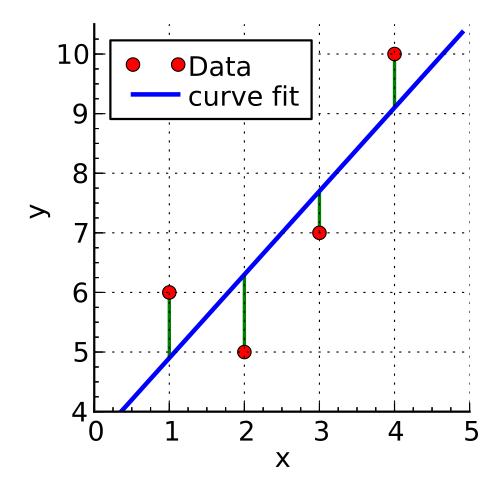
Suppose we have \(N\) data points \((x_i, y_i)\) and want to find the straight line \(y = mx + b\) that fits them as closely as possible. The least squares method finds the slope \(m\) and intercept \(b\) that minimize the sum of the squared vertical distances (shown below in green) between the data points and the line, using these formulas:

Figure 30.1. A least-squares line of best fit through four data points, with vertical distances (residuals) shown in green

\(\displaystyle m = \frac{N \sum(x_iy_i) - \sum(x_i) \sum(y_i)}{N \sum(x_i^2) - \left(\sum(x_i)\right)^2}\)

\(\displaystyle b = \frac{\sum(y_i) - m\sum(x_i)}{N}\)

The example below plots a set of data points along with their least-squares line of best fit.

Compile and run the code below in your own C environment.

#include <stdio.h>
#include <stdlib.h>

int main(void){
    float x[] = {1.2, 1.9, 3.2, 3.8, 5.1};
    float y[] = {0.9, 2.0, 3.1, 4.2, 5.3};
	 float xsol[] = {0, 6};
	 float ysol[2];
    int i;
	 int size = 7;
	 float sumx = 0;
	 float sumy = 0;
	 float sumxx = 0;
	 float sumxy = 0;
	 float m, b;
    
    FILE *gfile;

	 for(i=0; i<size; i++){
		 sumx += x[i];
		 sumy += y[i];
		 sumxy += x[i]*y[i];
		 sumxx += x[i]*x[i];
	 }
	 m = (size*sumxy - sumx*sumy)/(size*sumxx - sumx*sumx);
	 b = (sumy - m*sumx)/size;

	 ysol[0] = m*xsol[0]+ b;
	 ysol[1] = m*xsol[1]+ b;
	 printf("the solution is m = %f and b = %f\n", m, b);

	 /* Plot results */
    gfile = popen("gnuplot", "w");

    fprintf(gfile, "set terminal png\n");
    fprintf(gfile, "set output 'plot_regression.png'\n");

    fprintf(gfile, "set title 'Function'\n");
    fprintf(gfile, "set xlabel 'time (seconds)'\n");
    fprintf(gfile, "set ylabel 'position (m)'\n");
    fprintf(gfile, "set grid\n");

    fprintf(gfile, "plot '-' title 'data points', '-' with lines title 'best fit'\n");
    //fprintf(gfile, "plot '-' with lines title 'data', '-' with lines title 'data 2'\n");
    for(i=0; i<size; i++){
        fprintf(gfile, "%f %f\n", x[i], y[i]); // coordinates x and y
    }
    fprintf(gfile, "e\n");

	 fprintf(gfile, "%f %f\n", xsol[0], ysol[0]);
	 fprintf(gfile, "%f %f\n", xsol[1], ysol[1]);
    fprintf(gfile, "e\n");

    pclose(gfile);

    return 0;
}

Prev Top Next